RAID 3 Implementation Using MD (Multiple Disks) Drive.

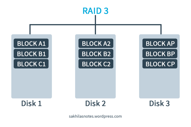
I’ve written about the RAID system and its techniques and levels in a previous entry. Please Click Here! In this article I am discussing a RAID 3 implementation using the tool called MD (Multiple Disks) Driver; AKA the Software RAID.

Software RAID vs. Hardware RAID

There are two possible approaches in implementing RAID: Hardware RAID and Software RAID. Software RAID (S/W RAID) implements the various RAID levels in block devices. It is the cheapest solution. Because here expensive hardware devices such as disk controller cards or hot-swap chassis are not required. S/W RAID also works with cheaper IDE disks as well as SCSI disks. With today’s fast CPUs, S/W RAID systems can perform better than Hardware RAID.

But anyways, S/W RAID comsumes the CPU cycles from the Processor of the host. In larger scale scenarios this can lead to many problems. The Hardware RAID (H/W RAID) manages the RAID subsystem independently from the host with the use of dedicated hardware devices to handle the operations. In this, host sees only a single disk per RAID array.

Back to work! In this S/W RAID implementation, I use 3 disks for the data and a additional one disk as a Hot Spare. A Hot Spare is a backup component that can be placed into service immediately when a primary component fails.

The MD driver provides virtual devices that are created from one or more independent underlying devices. In other words; after implementing the this RAID 3 system, it will be shown as a single disk to the user. But there are 4 underlying disk drives which actually hold the data.

For this implementations, firstly we have to install the tool MDADM (MD Administrator) to the system. We can do this using a simple YUM command.

# yum install mdadm

Then we have to select a set of disks/partitions for the RAID 3 system. For this we need 3 volumes as primary devices and another as the hot spare. The importance is, if the requirement is a RAID disk with the capacity of 4GB; the selected for volumes we selected should be equals or greater than 4GB. Let’s say we use the followings for the task.

/dev/sdb1       4GB
/dev/sdb2       4GB
/dev/sdc        4GB
/dev/sdd        4GB

Then we can create the RAID 3 Disk using the mdadm command. Here; we can either define the Hot Spare in the creation itself or create the RAID Disk without a hot spare.

# mdadm --create /dev/mda --level=3 --raid-devices=3 /dev/sdb1 /dev/sdb2 /dev/sdc
or
# mdadm --create /dev/mda --level=3 --raid-devices=3 /dev/sdb1 /dev/sdb2 /dev/sdc --spare-devices=1 /dev/sdd

The options in the command stand for the followings;
   –create defines the creation the RAID disk (mda)
   –level defines the RAID level
   –raid-devices defines the disks/partitions for primary devices
   –spare-devices defines the disks/partitions for spare devices

Then as we do with normal disks/partitions, we should install a file system to the RAID disk and mount it to a mount point.

# mkfs.ext4 /dev/mda
# mkdir /raidDisk
# mount /dev/mda /raidDisk

Now the user can access the RAID Disk mda via the /raidDisk mount point, treating it as a normaly mounted disk. User has no idea about the underlying disk arrengement. You can display the details about the RAID Disk arrengement using the following command.

# mdadm --detail /dev/mda

Data Recoverying Process in a Disk Failure

We can test the functionality of the RAID system by failing a primary device. In this case there are two scenarios. First is where you have a Hot Spare. The other scenario is when you have not configured a Hot Spare. First let’s see how to fail a drive.

# mdadm --manage /dev/mda --fail /dev/sdb1

With the above command now the drive sdb1 is failed. If there is a Hot Spare drive, now automaticall the lost data will be recovered in to it, the drive sdd.

If a Hot Spare is not assigned; the administrator should quickly remove the failed drive from the RAID system. It can be done using the following command;

# mdadm --manage /dev/md0 -r /dev/sdb1

Then the administrator should manually add a Spare Drive which is equal or greater than 4GB. Then quickly RAID system will start the recovering process. We can add a Spare drive (sde) to the system with the following command;

# mdadm --manage /dev/md0 -a /dev/sde

Either way is possible. To monitor the recoverying process we can display the MD Statistics using the following command.

# watch -n1 cat /proc/mdstat

What is  a Hot Spare Drive and a Spare Drive?

Hot Spare drive is a pre defined disk drives with the relevant requirements (such as capacity) and it works automatically in a drive failure. And a Spare drive is another disk drive with the relevant requirements and it is not pre defined. In case of drive failure; administrators can manually add the drive to the RAID system.

Remove a RAID Disk.

Under this sub topic lets discuss how to remove a RAID disk from the system and free the underlying disks/partitions. For this first we can check for the existing RAIDs using the following command.

# cat /proc/mdstat

The we need to unmount the RAID device.

# umount /dev/mda

Then we need to stop and remove the RAID array from the system. After executing this; the RAID controller will release the processes relevant to the particular RAID disk.

# mdadm --stop /dev/md0 mdadm --remove /dev/md0

To check for RAID dedicated underlying disks/partitions we can use the following command.

# lsblk -o NAME,SIZE,FSTYPE,TYPE,MOUNTPOINT

To release those disks/partitions we can follow the following commands;

# mdadm --zero-superblock /dev/sdb1
# mdadm --zero-superblock /dev/sdb2
# mdadm --zero-superblock /dev/sdc
# mdadm --zero-superblock /dev/sdd

By following this note; you will be able to configure a software RAID Disk successfully. With the practical approach only you can understand somethings in deap.

Good Luck & Have Fun!

What is RAID? How it works?

RAID (Redundant Array of Independent Disks; originally Redundant Array of Inexpensive Disks) is a way of protecting data against drive failure, by storing the same data in different places on multiple hard disks. Basic techniques, used in RAID are as follows;

Striping
Mirroring
Parity

RAID has an infinite number of implementations and the basic, more common implementations are as follows;

RAID 0

This is based only on Striping. This system can be implemented using a minimum disk count of 2. This implementation does not provide any protection against disk failure.

RAID 1

RAID 1 is based only on mirroring. Because of that it can protect data against single disk failure. Minimum disks needed is 2.

RAID 3

This system uses two techniques; striping and parity. One disk is dedicated for the parity. This system can protect data against single disk failure. At least 3 disk drives are needed.

RAID 5

This is so similar to RAID 3. The only difference here is, it does not use a dedicated disk for the parity. The parity is distributed among all the disks.

RAID 6

Very similar to RAID 5. But this uses 2 parities distributed into 2 separate disks. Because of this, RAID 6 can guarantee the protection of data against 2 disk failures.

RAID 1+0 (10)

This is a combined RAID system. It is designed using the concepts of RAID 1 and RAID 0. This system can protect your data against 2 disk failures. But more importantly, it cannot guarantee.

For an example: if Disk 1 and Disk 2 failed, the lost could not be recover.

RAID 0+1 (01)

Very similar to RAID 1+0, but the pattern in which RAID 1 and RAID 0 has been used is changed. This also cannot guarantee the data protection against 2 disks failure. But in some scenarios it can.

The basic idea behind RAID is this. We can choose any of the above levels of RAID in implementations. I will do a software level RAID 3 Implementation on a RHEL platform in my next post.

Good Luck & Have Fun!

SAN Implementation on a RHEL Platform

SAN stands for Storage Area Network. It is a dedicated high-speed network/subnetwork that interconnects and presents shared pools of storage devices to multiple hosts in the network. SAN server is called the Target and the clients are called Initiators. Storages are served as Blocks by the Target to its Initiators. In this post, I am configuring a SAN system using iSCSI.

iSCSI (Internet Small Computer System Interface) is a transport layer protocol which describes how SCSI (Small Computer System Interface) packets should be transported over a TCP/IP network. As the Target and Initiator, I’m using two RHEL7 VMs named RH.SANSVR and RH.SANCLI. The configurations of the iSCSI Target and a iSCSI Initiator are as follows;

RH.SANSVR: iSCSI Target Configuration

First, we should connect some hard disks to the system (In coop environment, storage arrays are used.) and decide which disks and partitions are to be used for the SAN system. Connected disks and their partitions can be listed using the following command;

# lsblk

Then, we should create Logical Volumes (LVs) using Logical Volume Manager (LVM) with the selected disks and partitions. If you do not know how to create LVs, Click Here!

Create a Volume Group (VG) named vg_iscsi. All the VGs can be listed using vgs/vgdisplay commands. Now create a LV named lv_disk0 from the created VG. These LVs are the storage portions which are going to be distributes through the internet to initiators.

Then as a best practice after doing a YUM (Yellowdog Updater Modified) update, install Target CLI (targetcli) to the system. It is the single-node LinuxIO management shell by Datera, Inc. We are going to use this CLI for our configurations.

# yum update
# yum install targetcli -y

After a successful installation switch to the Target CLI using the following command. Then inside that CLI if we execute the command ls, the directories inside the CLI will be listed.

# targetcli
>
> ls
o- / ............................................................... [...]
 o- backstores ..................................................... [...]
 | o- block ......................................... [Storage Objects: 0]
 | o- fileio ........................................ [Storage Objects: 0]
 | o- pscsi ......................................... [Storage Objects: 0]
 | o- ramdisk ....................................... [Storage Objects: 0]
 o- iscsi ................................................... [Targets: 0]
 o- loopback ................................................ [Targets: 0]

Then create a block storage object in the directory /backstores/block/ named iscsi_disk0, with the LV you created.

> cd backstores/block
> create iscsi_disk0 /dev/vg_iscsi/lv_disk0

Now create a WWN (World Wide Name) named as an IQN (iSCSI Qualified Name). This should be done inside the iscsi directory.

> cd /iscsi> create iqn.2017-08.iscsi.target:disk0

Here, if you just execute the command create, the WWN will be created with a default IQN. After creating this, if we execute a ls command inside the iscsi directory the result will be as follows;

> ls /iscsi/
o- iqn.2017-08.iscsi.target:disk0 ............................... [TPGs: 1]
 o- tpg1 ........................................... [no-gen-acls, no-auth]
   o- acls ...................................................... [ACLs: 0]
   o- luns ...................................................... [LUNs: 0]
   o- portals ................................................ [Portals: 0]

Inside the WWN there are three directories as ACLs (Access Control Lists), LUNs (Logical Unit Numbers) and Portals. In here, inside acls/ we should create a ACL with the WWN of the initiator.

> cd /iscsi/iqn.2017-08.iscsi.target:disk0/tpg1/acls
> create iqn.1994-05.com.redhat:node0

To find the IQN of the Initiator, use the following file in a iSCSI Initiator Utilities installed system.

# cat /etc/iscsi/initiatorname.iscsi
~ InitiatorName=iqn.1994-05.com.redhat:node0

Then inside luns/ we create a LUN with the block object we created previously.

> cd /iscsi/iqn.2017-08.iscsi.target:disk0/tpg1/luns
> create /backstores/block/iscsi_disk0

Then inside the portals/ we should create a portal using the IP address. This portal will use 3260 as the port address by default.

> cd /iscsi/iqn.2017-08.iscsi.target:disk0/tpg1/portals
> create 192.168.8.104

After those configurations, inside of the /iscsi directory will be shown as follows;

> ls /iscsi/
o- iqn.2017-08.iscsi.target:disk0................................ [TPGs: 1]
  o- tpg1 .......................................... [no-gen-acls, no-auth]
    o- acls ..................................................... [ACLs: 1]
    | o- iqn.1994-05.com.redhat:node0 .................... [Mapped LUNs: 1]
    |   o- mapped_lun0 ...................... [lun0 block/iscsi_disk1 (rw)]
    o- luns ..................................................... [LUNs: 1]
    | o- lun0 ................ [block/iscsi_disk0 (/dev/vg_iscsi/lv_disk0)]
    o- portals ............................................... [Portals: 1]
      o- 192.168.8.104:3260 .......................................... [OK]

Save the configurations and exit.

> saveconfig
> exit#

Then enable the target service at the startup, and restart the service.

# systemctl enable target.service
# systemctl restart target.service

Permenent the service port at the Firewall and reload firewall services.

# firewall-cmd --permanent --add-port=3260/tcp;
# firewall-cmd --reload

Now the Target is successfully configured, up and running. Now let’s look at the iSCSI Initiator, RH.SANCLI. the configurations are as follows;

RH.SANCLI: iSCSI Initiator Configuration

First, we should check the existing disks and their partitions using the following command. Because after successfully configuring the Initiator, the new block storages should be listed here.

# lsblk

Then, after a YUM update, install the iSCSI Initiator Utilities to the system.

# yum update
# yum install iscsi-initiator-utils -y

Using iscsiadm (Open-iSCSI Administration Utility) command line tool, things like allowing discovery and login to iSCSI targets, as well as access and management of the open-iscsi database can be done. Now we have to discover the target.

In iscsiadm tool’s options, –mode (-m) specify the mode. In discoverydb and node modes, all their respective records are displayed. In discoverydb mode there are different types. –type (-t) specifies the type, which is sendtarget in here. It’s a native iSCSI protocol which allows each iSCSI target to send a list of available targets to the initiator. –portal (-p) specifies the target portal with IP address and port number. –discovery (-D) is to command to start discovering the targets.

# iscsiadm --mode discoverydb --type sendtargets --portal 192.168.8.104 --discover

Then have to log in to the SAN Target. If the login is successful, the new disks should be available after executing lsblk. In this command, –mode is node. –targetname specifies the IQN of the target. –login is the commanding option.

# iscsiadm --mode node --targetname iqn.2017-08.iscsi.target:disk0 --portal 192.168.8.104:3260 --login

iscsiadm command line tool has many options available. To study these options please Click Here.

Then enable the initiator service at the startup, and restart the service.

# systemctl enable iscsid.service
# systemctl restart iscsid.service

If you want to logout from the target you can use the following command with –logout option;

# iscsiadm --mode node --targetname iqn.2017-08.iscsi.target:disk0 --portal 192.168.8.104:3260 –logout

After following this scenario; anyone with a basic knowledge of RHEL platform can configure a SAN system with a single target and an initiator. Practice more, and start doing experiments. Then only you will be able to work easily in Linux environments.

Good Luck & Have Fun!

Logical Volume Manager in RHEL

In Linux, Logical Volume Manager (LVM) is a device mapper that provides logical volume management for the Linux kernel. Most modern Linux distributions are LVMaware to the point of being able to have their root file systems on a logical volume.

Why LVM? Think of a scenario where you need three separate volumes, each is 3GB in size to save log files of two different applications. You have two free partitions of 2GB each in size. Altogether you have 4GB.  But as the requirement is two partitions which are 3GB each in size, you have to buy a 6GB storage disk, divide it into two and make two partitions. With this solution, the 4GB disk space is wasted.

This is where LVM comes to the scene. With LVM, you get the ability to buy only a 2GB new storage disk instead of buying a 6GB disk and create a Logical Disk of 6GB by adding the existing two Physical Partitions and the new Physical Disk together. Then you can create Logical Partitions of this logical disk as you needed.

I am discussing how to create Logical Volumes using Physical disks/partitions in this article. If you successfully followed this scenario, you’ll be able to understand and use LVM easily. This exercise is done in a RHEL 7 VM.

Logical Volume Creation

First, we should connect some hard disks to the system (In coop environment, storage arrays are used.) and decide which disks and partitions are to be used for the SAN system. Connected disks and their partitions can be listed using the following command;

# lsblk

Then, we should create Logical Volumes (LVs) using Logical Volume Manager (LVM) with the selected disks and partitions. For that, first we should label them as LVM Physical Volumes (PVs). I’m using two partitions as sdb1, sdb2 and a disk as sdc. All the PVs can be listed using pvs/pvdisplay commands.

# pvcreate /dev/sdb1 /dev/sdb2 /dev/sdc
# pvs
# pvdisplay

Create a Volume Group (VG) named vg_a. All the VGs can be listed using vgs/vgdisplay commands.

# vgcreate vg_a /dev/sdb1 /dev/sdb2 /dev/sdc
# vgs
# vgdisplay

Now create LVs named lv_a1 and lv_a2 from the created VG. These LVs are the storage portions which are going to be distributes through the internet to initiator. In this command -L property holds the size of the LV and -n holds the name. All the LVs can be listed using lvs/lvdisplay commands.

# lvcreate -L 2G -n lv_a1 /dev/vg_a
# lvcreate -L 2G -n lv_a2 /dev/vg_a
# lvs
# lvdisplay

As you can see, the second logical volume cannot be created with the size of 3GB because of insufficient disk space. Because of that the LV is created in the size of 2.5GB.

Good Luck & Have Fun!

Local Storage Disk Management in RHEL

With this article i am writing about the basics of local disk management in a RHEL (Red Hat Enterprise Linux) environment. Local disk management is about managing storage disk drives which are locally connected, or in other words physically connected to the system. Basic things in storage disk management such as naming convention of disk drives, disk partitioning and disk mounting is noted here.

Naming Convention

In Linux, every hardware device in listed under the directory /dev as files. Hard disk drives are also listed as files inside this directory. If we list all the files inside /dev directory, it will be something like this;

In here, every connected device to the system should have a clearly named file for the ease of the users. Basic naming structure of a storage disk drive is as follows;

[Protocol+Disk][Disk Number][Partition Number]

Ex: sdb1       [SCSI Disk][Disk B][Partition 1]

The type of the disk drive is describes with the first two letters as [Protocol+Disk]. First letter specifies the Linux I/O protocol which is used to configure the disk and the second letter, d stands for disk. Some commonly used protocols are as follows;

sd        SCSI based Disk

hd       ATA based Disk

vd       VirtIO based Disk

Third letter specifies the Disk Unit. The first disk attached to the system is named with the letter a, the second with b and so on. After naming the 26^th disk with z, the 27^th will be names as aa, next as ab and so on.

Last letter is to specify the partition number. This is done using numbers instead of letters. So the 1st partition of the disk b will have b1 as its third and fourth letters. For the ease of understanding, let’s have a look at the following examples;

sda      SCSI based Disk A

hdc2   ATA based Disk C’s 2^nd Partition

Knowing the naming convention is very important, because in storage disk management, knowing the names of the disks that you are dealing with will be very helpful. You will understand it with following exercises.

Storage Disk Partitioning

A storage disk can be divided into several storage units which are called partitions. By creating partitions we can treat one physical storage drive as multiple drives. This task is done on a RHEL 7 Virtual Machine. In Linux, we call storage disks as Blocks. We can list all the available block drives using the lsblk command;

# lsblk

Then to partition a disk, we use the command line tool; fdisk. FDisk (Fixed Disk/Format Disk) is a commonly used command line based disk manipulation utility for a Linux/Unix systems. With this, you can view, create, resize, delete, change, copy and move partitions on a storage disk drive.

Now let’s try to partition a SCSI based 4GB disk named as sdb.

# fdisk /dev/sdb

After executing this command, the console will be changed to the fdisk console. By default it says to enter m for help. If we input m and press enter, a list of fdisk commands will be displayed. As an example we can enter p to the console to view all the partitions in the partition table.

To create a new partition, we are going to use the command n. This stands for creating a new partition. After inputting n to the fdisk console, a partitioning wizard will be started. We are required to input some properties to the wizard in order to create the partition we need.

The first property is the type of the partition. Mainly there are two types of partitions as Primary partitions and Extended partitions. So, what is the difference between these two types?

Primary and Extended Partitions

Only Primary partitions can hold the Boot files of a system. A single disk can only have a maximum number of four primary partitions. If there are multiple primary partitions, the one who holds the boot files should be marked as Active. So, the BIOS will search for the boot files in the active primary partition. Extended partitions cannot be marked as active.

A single disk can only have one Extended partition. That means, a single disk can be divided into either four primary partitions or three primary partitions and one extended partitions. But, extended partitions can be subdivided into several partitions which are called Logical partitions.

Basically, Primary partitions are bootable partitions which hold the OS of a system, while extended partitions are not bootable but can be used to store data. So, in creating a new partition, we should input whether we are going to create a primary partition or an extended partition. By default, primary partitions are named using number 1 to 4 (1-4).

Then as the second property, we need to input the first cylinder of the partition. This is to specify the cylinder of the hard disk which is going to be the first cylinder of he partition. It’s always better to go with the default value.

Then the last cylinder of the partition is requested by the wizard. If we specify a cylinder here, the space between that cylinder and the first cylinder will be taken as the partition. And we also can just input the size of the partition which needs to be created. Then the system will do the math for you and calculate the last cylinder number by itself. To input the size, we can use K (for Kilobytes), M (for Megabytes) or G (for Gigabytes) along with a “+ sign” as follows;

Last cylinder: +1000B , +100M or +1G

After that the wizard will be finished and the partition is created. But prior exiting the fdisk console, we should write all the changes to the partition table. For this we can enter w to the console.

Now we can list the available blocks again using the lsblk command and see whether the partitioning is successful.

To use the block storage to store directories and files, a file system should be installed. In a system, a file system is the way in which files are named and where they are placed logically for storage and retrieval. To install a file system, the command mkfs (Make File System) is used. There are many commonly used file systems such as ExtN, XFS, Exbibyte, etc. and in this scenario Ext4 is used.

# mkfs.ext4 /dev/sdb1

After installing a file system, now the block storage can handle files. But still, it is not yet connected to the Root (/) file system wich exists in the Active Primary partition, or in other words; we still do not have a path to access the storage. So, we should create a directory, somewhere in the root filesystem and the disk/partition should be mounted to it. This is called a mount point.

# mkdir /mountSdb1
# mount /dev/sbb1 /mountSdb1

Now on, all the directories and files which is stored inside /mountSdb1, is stored inside sdb1. To check the block id, use the following command.

# blkid /dev/sdb1

After successfully completed this note, you should be able to manage the connected storage disk drives of your system like a pro.

Good Luck & Have Fun!